Laffer Curve

**higher the tax rate you set, less $ you will collect
**Laffer Curve is controversial and debatable


*trade-off b/t tax rates and govt revenue
*as tax rates ↑ from 0, tax revenues ↑ from 0 to some max level, and then decline
*higher tax rates, less $ you collect
*Criticisms:

1. where economy is located on curve, it is difficult to determine
2. tax cuts also ↑ demand which can fuel inflation
3. empirical evidence suggests that impact on tax rates on incentives to work, save, and invest are small

Phillips Curve Cont.

SRAS→=SRPC←

(imagine the direction of the arrows on the corresponding graphs below)

• inflationary expectations ↓, input prices ↓, productivity ↑, business taxes ↓, +/or deregulation
• SRAS→: GDPR↑ and PL ↓; u%↓ and π%↓
• SRPC← (disinflation)

 *supply shock→rapid and significant increase in resource cost which causes the SRAS to shift

*NRU→is = to frictional, structural, and seasonal (cyclical based on economy)

• natural rates and fewer worker benefits create a lower NRU (free med. care for all workers, lay-off some b/c profits being eaten)

*misery index→combo. of inflation (2-3%) and unemployment (double digits=depression, forget a recession) in any given year. Single digit misery is good. 

*if inflation rate persists and expected rate of unemployment rises, then entire SRPC moves upward. When that happens, stagflation exists. 

*if inflation expectations drop (due to new tech., efficiency, etc.), the SRPC moves downward

*stagflation→↑ unemployment and ↑inflation occurring at same time

*disinflation→when inflation decreases over time 

• nominal wages ↓ (good)
• business profits fall as prices ↑ (bad)
• firms reduce employment, thus, unemployment ↑

Unit VI: The Phillips Curve

u%=unemployment rate
π%=rate of inflation

*The Phillips Curve represents the relationship b/t unemployment and inflation
*trade-off b/t unemployment and inflation occurs over SR
*each point on the Phillips Curve corresponds to a different level of output
*LRPC=long run Phillips Curve

• occurs at NRU

• represented by ↨ line

• no trade-off b/t unemployment and inflation in LR

1. economy produces @ FE output level
2. nominal wages of workers fully incorporates any changes in PL as wages adjust to inflation over the LR

*LRPC only shifts when LRAS shifts (both have the same determinants)
*↑ in unemployment, LRPC →
*↓ in unemployment, LRPC ←
*Increase in AD=up/left movement along SRPC 

• C↑, Ig↑, G↑, and/or Xn↑
• AD→: GDPR↑ and PL ↑; u%↓ and π%↑; up/left along SRPC
• this would be depicted in the graph below 

*Decrease in AD=down/right along SRPC

• C↓, Ig↓, G↓, and/or Xn↓
• AD←: GDPR↓ and PL↓; u%↑ and π%↓; down/right along SRPC
• in this case, point B would move to point A in the graph below

**Check out this blog for more info. on the Phillips Curve and other economic topics: http://macroeconomic1.wordpress.com/ 

Unit V: AD/AS: From SR to LR

*AS curve doesn't shift in response to changes in the AD curve in the short run

• i.e.-nominal wages do not respond to PL changes
• workers may not realize impact of the changes or may be under contract (i.e. teachers don't get paid more for tutorials)

*Long run (vertical)-prd in which nominal wages are fully responsive to previous changes in PL

*when changes occur in the SR, they result in either increased/decreased producer profits-not changes in wages paid

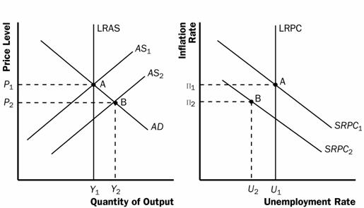
*in the LR, increases in AD result in a higher PL. As in SR, but as workers demand more $, the AS curve shifts left to equate production @ the original output level, but now @ a higher price. 

*in the LR, the AS curve is vertical (LRAS) @ the natural rate of unemployment (NRU), or FE level of output. Everyone who wants a job has one and no one is enticed (lured or tempted) into or out of market.

*Demand-pull inflation will result when an increase in demand shifts the AD curve to →, temporarily increasing output while raising prices. 

*Cost-push inflation results when an increase in input costs that shifts the AS curve to ←. In this case, the PL increase is not in response to ↑ in AD, but instead the cause of PL increasing. (in a recession, AD ↓ and shifts ←)

Graph: Crowding Out

Monetary & Fiscal Policy (during a recession)

Monetary Policy (Recession)	International Trade
Fed will:       1.       Buy bonds                       2.       Lower RR                       3.       Lower DR       4.       Lower FF  all contribute to: MS ↑, i ↓, Ig ↑, AD ↑, GDP ↑ **opposite occurs during inflationary prd	D $ (demand for $) ↓ ↓ $ depreciated (value of $ goes ↓) ↓ Exports ↑ (cheaper) ↓ Xn ↑ ↓ AD ↑ ↓ GDP ↑

Fiscal Policy (Recession)	International Trade
-congress will cut taxes or ↑ govt spending -consumption and govt spending will ↑ -AD will ↑ -GDP ↑ -Deficit→supply of LF ↓ (none to loan out) ↓ I (interest) ↑ Ig ↓	D $ ↑ ↓ $ appreciate (increase in value) ↓ Exports ↓ ↓ Net exports ↓ ↓ AD ↓ ↓ GDP ↓

Loanable Funds Market

Loanable Funds Market (LF)→market where savers and borrowers exchange funds (QLF) @ real rate of interest (r%)

• D for LF, or borrowing comes form households, firms, govt, and foreign sector. DLF is supply of bonds

• SLF, or savings comes from households, firms, govt, and foreign sector. SLF also demand for bonds. 

Changes in DLF:

• more borrowing=more demand for LF (→)
• less borrowing=less demand for LF (←)

EX) Govt deficit spending=more borrowing

• =more DLF (DLF→, r% ↑) 

 less investment demand=less borrowing

• less DLF (DLF ←, r% ↓)

Changes in SLF:

• more saving=more SLF (→)
• less saving=less SLF (←)

EX) Govt budget surplus=more saving

• more SLF (SLF →, r% ↓)

Decrease in consumer's MPS=less saving

• less SLF (SLF ←, r% ↑)